Radiochromic.com implements state-of-the-art models and computations to make radiochromic film dosimetry, image analysis, and machine QA easy, fast, and accurate.
Read and follow these Tutorials carefully to obtain the most accurate results.
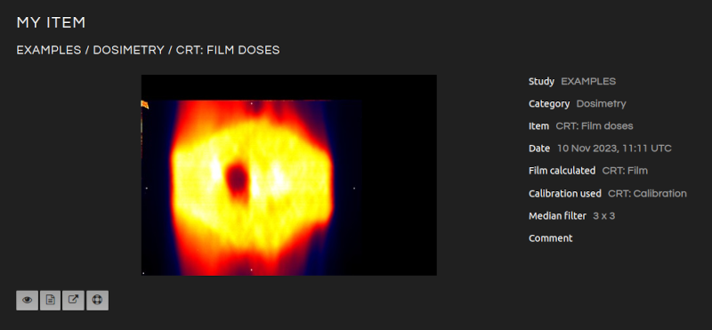
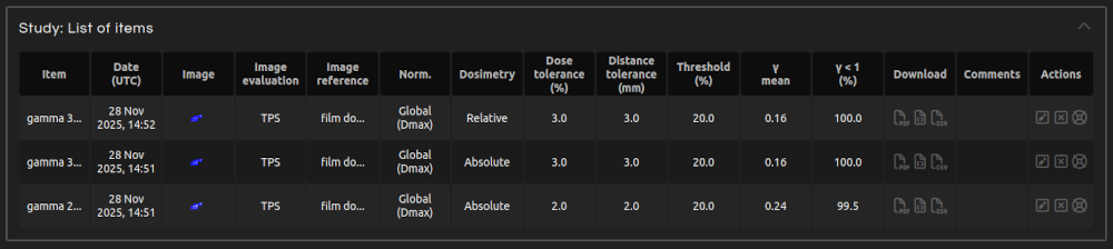
Explore all your imported and calculated items in My Work.
- My Work:
- Open MY WORK in the menu. Alternatively, click on the Radiochromic.com logo to open My Work.
- Study: Selection
- Select a list of items by Study type, Study, and Category. Study types include Active, Archived (studies accessible only in My Work), and Examples (demo studies for testing).
- Load / Refresh
- Load your selected list of items. Click Refresh to update it if a calculation was in progress.
- Edit:
- Rename a study
- Archive / Restore:
- Archive studies if you do not want to select them for new calculations. Archived studies are only accessible in My Work. Click Restore to make them Active again.
- Delete:
- Click Delete to permanently remove a study and all items within it.
- Edit item:
- In the Actions column of an item, click the Edit button to modify the Study, Item, or Comment.
- Delete item:
- In the Actions column of an item, click the Delete button to permanently remove it.
- Request item support:
- In the Actions column of an item, click the Support button to request support for this item.
To import images into Radiochromic.com, a subscription is required. For more information, please contact us.
Radiochromic.com does not record or use patient data. Do not enter patient data to identify items or studies.
Import film scans to Radiochromic.com.
- Step 1:
- Open IMPORT in the menu.
- Step 2:
- Click Film.
- Step 3:
- Select an existing Study or create a new one.
- Step 4:
- Name the Item.
- Step 5:
- If several film scans are uploaded, the files will be combined into an average film for import. Select how the films are averaged: using either mean or median pixel values.
- Step 6 (optional):
- Enter film statistics. Statistics help describe your films and are used to improve the accuracy of your results.
- Step 7 (optional):
- Add comments if desired.
- Step 8:
- Upload one or several repeated film scans taken after irradiation. Up to five images can be imported, with a maximum of 10M pixels for each image.
- Step 9 (optional):
- Upload one or several repeated film scans taken before irradiation. Scans taken before and after irradiation should be registered for accurate calculations of film doses. Up to five images can be imported, with a maximum of 10M pixels for each image.
- Step 10:
- Select film orientation. This is CRITICAL if lateral corrections are applied. Click the arrows ( or ) to select the direction of movement of the scanner lamp across the film scans.
- Step 11:
- Click Upload. The average film scans will be calculated and uploaded. They will be saved in My Work.
Import dose planes or image maps (e.g., EPID images) to Radiochromic.com.
- Step 1:
- Open IMPORT in the menu.
- Step 2:
- Click Image 2D.
- Step 3:
- Select an existing Study or create a new one.
- Step 4:
- Name the Item.
- Step 5:
- Choose the format of your image file or let the application detect it automatically. Currently supported image formats are:
- DICOM-RT dose 3D slice
- DICOM-RT dose 2D
- DICOM-RT image
- TIFF image
- Comma Separated Values
- XiO and Monaco (Elekta)
- iPlan (Brainlab)
- ADAC Pinnacle (Philips)
- OmniPro I'mRT (IBA) .opg file
- Step 6 (DICOM-RT dose 3D slice only):
- If you select DICOM-RT dose 3D slice, you must specify a plane in the 3D dose matrix, and provide the DICOM coordinates of the plane.
- Step 7 (optional):
- Add comments if desired.
- Step 8:
- Add the image file. Images can be up to 10M pixels. DICOM-RT dose 3D matrices may be larger, but sliced images should also be less than 10M pixels. Only square pixels are currently supported.
- Step 9:
- Click Upload. The image will be uploaded and saved in My Work. Files are anonymized upon upload.
Contact user support if your TPS / 2D dosimeter is not listed.
- ADAC Pinnacle (Philips):
- Planar Dose Computation -> Export Planar Dose -> Format: ASCII (Resolution: cm, Dose Units: Gy)
- Eclipse (Varian):
- Export dose plane → Dose absolute, Planar dose: 512 points, Burn marker pixels: No
- iPlan (Brainlab):
- Export → Dose → Select region, Dose Range and Step
- Monaco and XiO (Elekta):
- Dose profile → Image 2D output
- MultiPlan (Accuray):
- Plan → Export DICOM Data → Planar Dose
- OmniPro I'mRT/I'mRT+ (IBA) - ASCII .opg file:
- Export Data → Generic ASCII File → Entire file
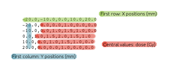
Import dose distributions in comma-separated values format. Doses should be in Gy and positions in mm. Follow the format of the example below:
Import several files together to Radiochromic.com.
- Step 1:
- Open IMPORT in the menu.
- Step 2:
- Click Series.
- Step 3:
- Select an existing Study or create a new one.
- Step 4:
- Name the Item.
- Step 5:
- Choose the format of your image files or let the application detect it automatically.
- Step 6 (optional):
- Add comments if desired.
- Step 7:
- Add the image files. Up to 400 images can be imported, each with a maximum of 10M pixels.
- Step 8:
- Click Upload. The images will be uploaded and saved in My Work. Files are anonymized upon upload.
Many different protocols for radiochromic film dosimetry can be applied with Radiochromic.com. Here, we present our recommended protocol for accurate radiochromic film dosimetry. This protocol is based on:
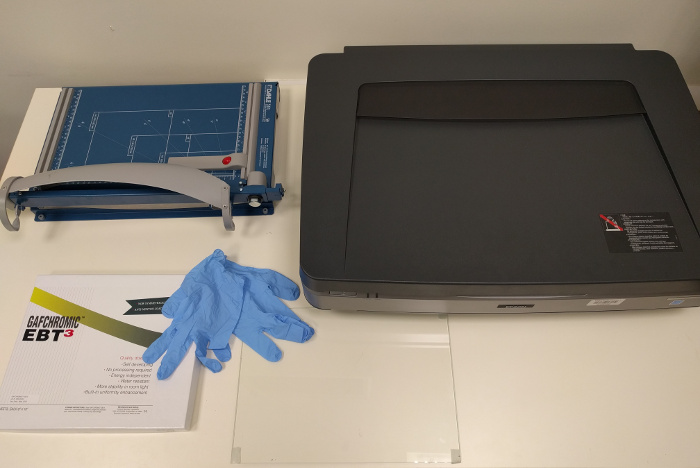
The dosimetry system for radiochromic film dosimetry consists of:
- Gafchromic radiotherapy/radiology films
- a flatbed scanner
- scanner software
- Radiochromic.com
The recommended accessories are:
- gloves
- a guillotine
- a frame to center the film on the scanner
- a transparent compression (glass) sheet, when scanning in transmission mode
- Keep films in a dry and dark environment.
- Handle films with care, do not touch them without wearing gloves to prevent marks and scratches.
- Keep films away from light whenever possible.
- If films are submerged in water, minimize the time of submersion.
- Do not bend films when cutting them. Use sharp scissors or, preferably, a guillotine.
- Films should always keep the same orientation (i.e., portrait or landscape) on the scanner. Mark each film or film fragment to keep the orientation with the original film sheet and place them consistently on the scanner.
- Step 1:
- Warm up the scanner (30-45 min).
- Step 2:
- Films, either entire films or film fragments, shall always keep the same orientation (i.e., portrait or landscape) on the scanner. Use the marks to place films consistently on the scanner.
- Step 3:
- Before acquisitions and after pauses, perform several (e.g., five) empty scans to stabilize the scanner lamp.
- Step 4:
- Center the film on the scanner. A convenient way to do so is with a frame.
- Step 5:
- Always use the same scanning mode, either reflection or transmission, that was used for the calibration.
- Step 6:
- Films shall be in perfect contact with the surface of the scanner bed to avoid curling. In transmission mode, place a 2-4 mm thick glass or PMMA sheet on top of the film. The positioning of the compression sheet shall be consistent; therefore, either cover or keep free the autocalibration area for all the scans. In reflection mode, the scanner lid itself compresses the film adequately.
- Step 7:
- Select the scanning area.
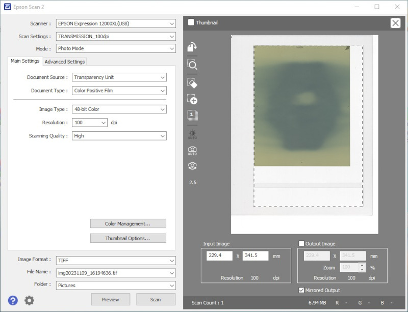
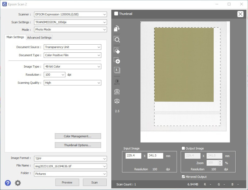
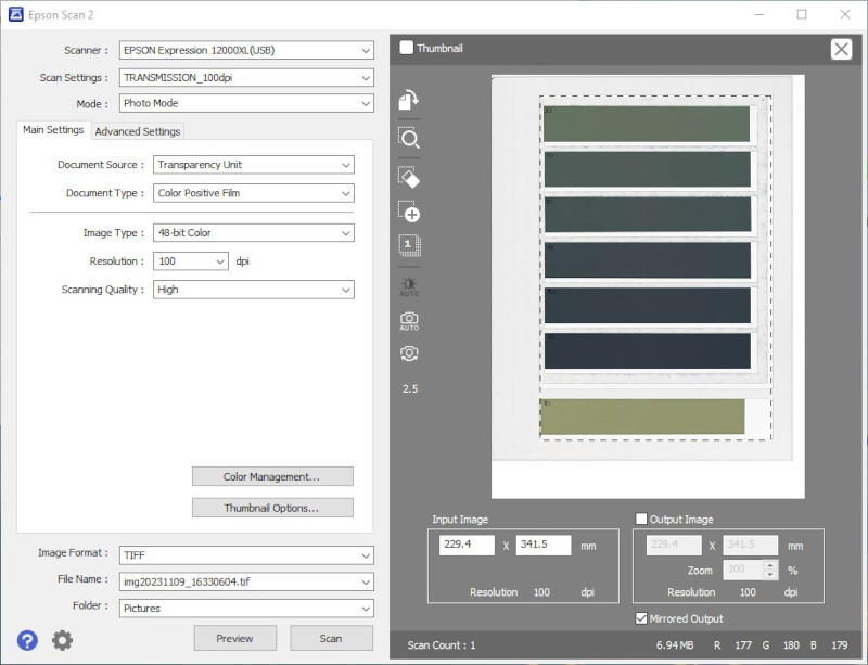
- Step 8:
- Acquire images with image type set to 48-bit RGB (16 bit per channel) and image processing tools turned off. Save the data as uncompressed TIFF files.
- Step 9:
- Perform four or five repeated scans and discard the first one for each film.
- Step 1 (optional):
- Prior to irradiation, scan the films that you will be using. If films are cut into fragments, scan them after cutting.
- Step 2:
- Irradiate the films.
- Step 3:
- Wait for the polymerization to stabilize and scan the films.
- Step 4:
- Upload the film scans to Radiochromic.com
A calibration is necessary to convert the response of the dosimetry system into a dose distribution.
In this protocol, we expose a calibration procedure for external photon beams, yet, other methods, radiation sources, and applications are possible, provided that they observe four basic principles:
- Calibrations are valid for films from the same lot; therefore, each lot of films has to be calibrated at least once. However, since films slowly autopolymerize over time, it is advisable to repeat lot calibrations from time to time. Furthermore, since film response depends on humidity and temperature, more accurate film doses can be expected when calibration and film dose measurements are done together.
- Uncertainties in the absorbed reference doses will be translated into film dose uncertainties. Hence, it is important to maximize the accuracy of the reference doses and select ROIs with homogeneous doses.
- To avoid the lateral response artifact, the ROIs with reference doses should be centered on the scan.
- The reference doses should cover the range of doses of interest to prevent extrapolations.
- Step 1 (only with lateral correction):
- If the calibration will include the lateral correction, acquire the image of an entire unexposed film. Unexposed films do not have scans before and after irradiation, simply upload them as IRRADIATED scans.
- Step 2:
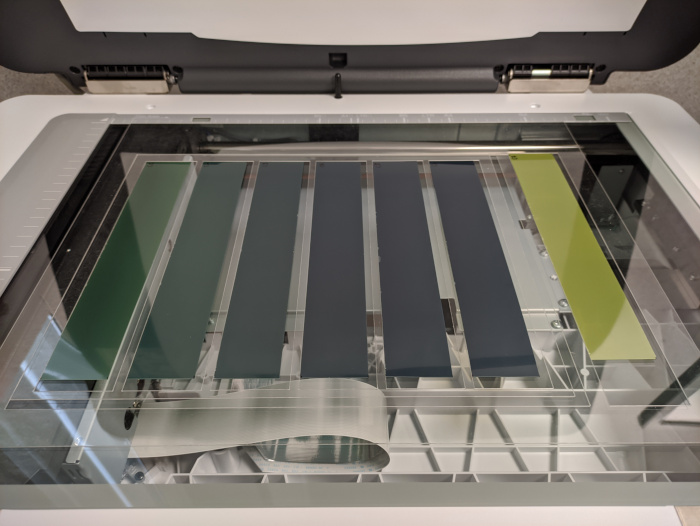
- Cut a film into several (e.g., seven) strips with the longer side of the strips parallel to the lamp.
- Step 3 (optional):
- Scan the film fragments prior to irradiation.
- Step 4:
- Irradiate all but one of the strips with known doses. The doses should go from 0 Gy (the unexposed film fragment) to approximately 120 % of the maximum dose of interest. If the calibration includes lateral correction, irradiate the strips with approximately homogeneous doses using a beam with a flattening filter and a 25 cm × 25 cm field. Additionally, if the calibration includes lateral correction, the scanning area should not be much larger than the length of the strips.
- Step 5:
- Scan all the calibration strips simultaneously. The irradiated areas of the strips should be centered on the scan.
- Step 6:
- Open FILM in the menu.
- Step 7:
- Click Calibration.
- Step 8:
- Select an image of a Calibration film.
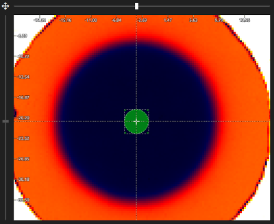
- Automatic ROI selection (optional):
- Automatic ROI selection can assist you with selecting the reference dose ROIs faster and more consistently. It is especially useful with unflattened fields (e.g., Cyberknife, ZAP-X, FFF fields, ...) to locate the center of the fields:
- Activate Add ROI centers.
- Enter the width and height of the ROIs. To provide enough statistics for the calibration while avoiding the lateral artifact, the height of the ROIs should be between 1-4 cm approximately.
- Set the approximate position of the ROIs by clicking with the left mouse button on the image display. The ROIs should be centered on the image (and on the scan).
- Click Apply. The application will find the centers of the fields and add centered ROIs.
- You may need to adjust the Threshold level to help the application with the automatic detection.
- If needed, you can repeat the process to add additional ROIs.
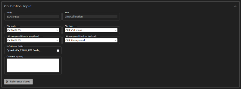
- Step 9 (Inputs):
- Enter the inputs for the calculation:
- Study:
- Select an existing Study or create a new one.
- Item:
- Name the Item.
- Select Channels:
- Choose the color channels to be used for the calibration. For better accuracy, we recommend using all three channels (RGB).
- Select Non-irradiated channels:
- If film scans taken before irradiation were imported, you can use them for the calibration as well.
- LRA: unexposed film (optional):
- To apply lateral corrections, select study and item of an imported unexposed film. Do NOT apply lateral corrections if the strips in your calibration film were not irradiated along their entire length.
- ROI geometry:
- Select between Rectangular and Elliptical ROIs. Circular ROIs (i.e., elliptical ROIS with equal width and height) are particularly useful for unflattened fields.
- LRA direction:
- Verify that the axis of the lateral response artifact (i.e., the axis parallel to the lamp) is shown as the Y axis in the image display. If that is not the case, rotate the image.
- ROIs:
- Associate reference doses to ROIs. The ROIs should be centered on the image (and on the scan). A minimum of three dose ROIs is required.
- Comments (optional):
- Add comments if desired.
- Step 10:
- Click Calculate. The calculation is in progress. The result will be saved in My Work.
- Step 11:
- You can modify the Calibration inputs to run multiple calculations in parallel.
- In My Work:
- Click on the Calibration item to open it in Image Analysis.
- Click on Image film or Image unexposed film to open them in Image Analysis.
- Download the calculation report as a PDF, CSV, or JSON file.

Convert film pixel values into doses.
- Step 1:
- Calibrate the film lot.
- Step 2:
- Irradiate, scan and upload the film.
- Step 3:
- Open FILM in the menu.
- Step 4:
- Click Dosimetry.
- Step 5:
- Select the image that you imported for dosimetry.
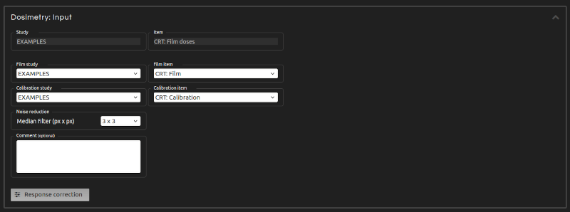
- Step 6 (Inputs):
- Enter the inputs for the dosimetry:
- Study:
- Select an existing Study or create a new one.
- Item:
- Name the Item.
- Calibration:
- Select the calibration for the dosimetry.
- Select Channels:
- Choose the color channels to be used in the calculation among those selected in the calibration.
- Select Non-irradiated channels:
- If film scans taken before irradiation were imported and the non-irradiated channels were included in the calibration, you can use them for dosimetry as well.
- Noise reduction:
- Noise reduction applies a square median filter to the dose distribution to reduce noise (a 3 × 3 filter is recommended).
- LRA direction:
- Verify that the axis of the lateral response artifact (i.e., the axis parallel to the lamp) is shown as the Y axis in the image display. If that is not the case, rotate the image.
- Inter-scan correction (optional):
- Select an unexposed ROI to correct inter-scan variations. Use the central part of the scan to avoid the lateral artifact. The unexposed film fragment from the calibration can be used to correct inter-scan variations. To do so, you may keep this fragment in the same position when scanning every film until a new calibration is performed.
- Dose rescaling (optional):
- Rescale doses in order to match the film dose with the known dose of a ROI. To apply dose rescaling, before the irradiation, cut a strip from the film to measure. This strip should be irradiated with a known homogeneous dose and scanned together with the rest of the film. Finally, select a ROI of the strip centered on the scan and enter its dose.
- Comments (optional):
- Add comments if desired.
- Step 7:
- Click Calculate. The calculation is in progress. The result will be saved in My Work.
- Step 8:
- You can modify the Dosimetry inputs to run multiple calculations in parallel.
- In My Work:
- Click on the Dosimetry item to open it in Image Analysis.
- Click on Image film to open it in Image Analysis.
- Click on Calibration to open it in My Work.
- Download the calculation report as a PDF, CSV, or JSON file.
Analyze imported and calculated images.
- Step 1:
- Open IMAGE in the menu.
- Step 2:
- Click Analysis.
- Step 3 (Image selection):
- Select one or two images or one series for display.
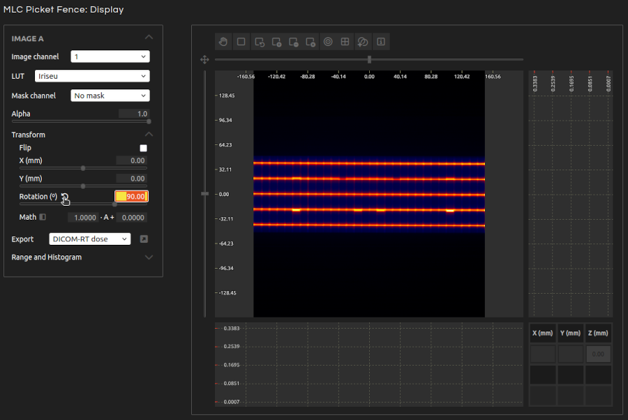
- Step 4 (Display):
- Manipulate and analyze your images, export them as DICOM-RT dose/image, export profiles, etc.
- Image handlers:
- Manipulate Image A, B, and Image Calculator. Image Calculator offers the possibility to calculate the image which is the difference (i.e., \(A - B\)), relative difference (i.e., \(100 \frac{A - B}{B}\)), or addition (i.e., \(A + B\)) of images A and B.
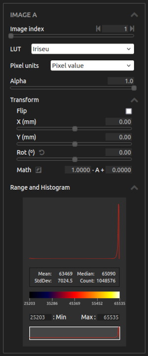
- Image channel / Image index:
- Select a channel in a Film or Image 2D, or an image within a Series. Only the first channel of each image is accessible for Series.
- LUT:
- Choose between different color lookup tables.
- Mask channel:
- Select a mask channel to exclude certain pixels from display.
- Alpha:
- Adjust the transparency/opacity level of the image.
- Transform:
- Apply affine transformations to the image. The order of transformations is: first Flip, then Rotation, and finally Translation. Math will multiply each pixel in an image by the first parameter and add the second parameter. Rotate in 90º steps by clicking on . Calculate the complement of the image by clicking on .
- Export:
- Export the image as DICOM-RT dose, DICOM-RT image, or TIFF image. TIFF images are exported as 16-bit integers. To preserve precision when exporting doses as TIFF files, it is recommended to scale images by 100 or 1000 to export in cGy or mGy. If a ROI is selected, only the ROI will be exported.
- Range and Histogram:
- Select the range of values of interest. Examine the distribution of values with the histogram and the statistical analysis. If a ROI is selected, only the points inside the ROI are included in the analysis.
- Display buttons:
- Customize the display.
- Move Image A:
- Drag Image A using the left mouse button instead of the middle mouse button by clicking on .
- ROI:
- Select Region of Interest with the left mouse button or by clicking the ROI button .
- Zoom:
- Zoom/unzoom using the right mouse button or the zoom buttons: .
- Isodoses/isolines:
- Show isodoses/isolines on the images with the Isodoses button .
- Grid:
- Show a grid on the canvas with the Grid button .
- Gamma registration:
- Register two images automatically through gamma index optimization .
- Marker registration:
- Use fiducial markers to displace an image or register it with another one .
- Information:
- Show the names of the images with the Information button .
- Sync Image B range to Image A range:
- Click the Sync button to synchronize Image B range with that of Image A.
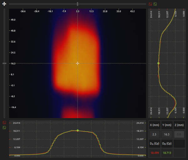
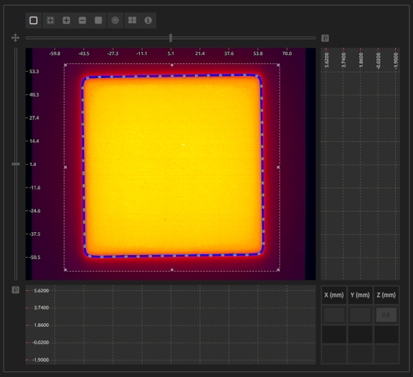
- Canvas:
- Visualize and analyze the image.
- Drag:
- Use the middle mouse button to drag the Image A.
- Cursor:
- Read pixel values under the cursor. Lock the cursor by clicking on . You can adjust the cursor position using the sliders located on the top and left sides of the canvas.
- Profiles:
- Vertical and horizontal profiles for both images are shown. Image A is in red, Image B is in green, and Image calculator is in blue. To export a profile, lock the cursor, select the Profile export step on the Image handler, and click on the Export button to export it in CSV format.
- Average profiles:
- Select a ROI and click the Average button to obtain the average profile. Click the Export button to export it in CSV format.
- Control area:
- Visualize pixel coordinates and pixel values in the control area. You can also move the cursor to a specific position by entering the coordinates in the control area.

Use fiducial markers to displace an image or register it with another one.
- Step 1:
- Select the image to be displaced.
- Step 2:
- Add as many markers as needed.
- Step 3:
- For each marker, define its From and To coordinates. From corresponds to the current location of the marker on the canvas, and To represents the desired final location. You can enter coordinates manually, or click on to place them directly on the canvas using the left mouse button. Zooming can help you position them more precisely. From coordinates always require both X and Y values, whereas To coordinates may contain only one dimension.
- Step 4:
- Click Apply. After a few seconds, the registration will apply an affine transformation to the image selected to minimize its distance to the specified To coordinates.
Register two images automatically through gamma index optimization.
- Step 1:
- Pre-register both images by flipping, translating, and rotating them.
- Step 2:
- Select which variables can be included in the registration: Translation X, Translation Y, Rotation Z, and Dose scaling.
- Step 3 (optional):
- Select the region to include in the registration using a ROI. Otherwise, the registration will use all pixels in both images.
- Step 4:
- Click Apply. After a few seconds, the registration will apply an affine transformation to Image A to register both images.
- Troubleshooting 1:
- If the images are too far apart from each other, or the rotation between them is too large, the registration will fail. Pre-register both images beforehand.
- Troubleshooting 2:
- The rotation may fail if one image has perfect circular symmetry.
- Troubleshooting 3:
- The registration expects similar dose distributions (in absolute or relative values). Registering images with similar shapes but completely different pixel values may lead to failure.
Compare dose distributions by evaluating the 2D γ-index.
- Step 1:
- Open IMAGE in the menu.
- Step 2:
- Click Gamma.
- Step 3:
- Select the evaluation (Image A) and reference (Image B) dose distributions.
- Step 4:
- If necessary, scale or increment the doses of Image A by a fixed value with Transform / Math. For example, if you are using a dose plane calculated by the TPS, you can input the daily output of the linac as dose scaling factor. If you are using a dose plane measured with a 2D dosimeter, you can introduce the necessary dose scaling factor to correct for the distance between the film plane and the dosimeter's measurement plane.
- Step 5:
- Pre-register both images by flipping, translating, and rotating them.
- Step 6 (optional):
- Register both images automatically with markers (Marker registration) or dose distributions (Gamma registration).
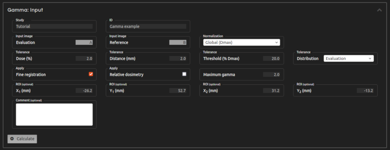
- Step 7 (Inputs):
- Enter the inputs for the calculation:
- Study:
- Select an existing Study or create a new one.
- Item:
- Name the Item.
- Normalization:
- Choose between global and local gamma normalization. Global gamma can be normalized at Dmax or at a specified Dnorm.
- Tolerance Dose:
- Select dose tolerance as a percentage of Dmax or Dnorm (for global normalization) or of the local dose (for local normalization).
- Tolerance Distance:
- Insert the distance tolerance in mm.
- Threshold:
- Specify the threshold dose. Points with doses lower than the threshold dose are excluded. The threshold dose is a percentage of Dmax or Dnorm.
- Ceiling (optional):
- Specify a ceiling dose. Points with doses higher than the ceiling dose are excluded. The ceiling dose is a percentage of Dmax or Dnorm.
- Tolerance Distribution:
- Select the distribution from which global gamma dose tolerances are calculated. You can use either the reference or the evaluation dose distribution.
- Maximum gamma:
- The maximum gamma value restricts the search space around each reference point. (Default: 2.0)
- Fine registration:
- If selected, the automatic fine registration will improve your registration to optimize the γ-index results.
- Relative dosimetry:
- If selected, the application will consider that the images contain relative doses. To optimize the γ-index results, doses in Image A will be scaled.
- Interpolation:
- Use bicubic interpolation on the evaluation image to increase the accuracy of the results.
- ROI (optional):
- Select the area to be included in the analysis.
- Comments (optional):
- Add comments if desired.
- Step 8:
- Click Calculate. The calculation is in progress. The result will be saved in My Work.
- Step 9:
- You can adjust the Gamma inputs to run multiple Gamma Index calculations in parallel. For example, you can modify tolerances, apply relative dosimetry, and then click Calculate again.
- In My Work:
- Click on the Gamma item to open it in Image Analysis. The resulting image includes Gamma, Gamma angle, and Mask. The Gamma angle is measured in degrees: angles close to 0° indicate mostly dosimetric errors, while angles near 90° indicate spatial mismatches. Points exceeding the maximum gamma are indicated by a Gamma angle value of 180°. The Mask excludes pixels not included in the calculation.
- Click on the images to open them in Gamma with registration applied.
- Download the calculation report as a PDF, CSV, or JSON file.
- References:
- Low, D. A., et al. "A technique for the quantitative evaluation of dose distributions." Medical physics 25.5 (1998): 656-661.
- Stock, M., et al. "Interpretation and evaluation of the γ index and the γ index angle for the verification of IMRT hybrid plans." Physics in Medicine & Biology 50.3 (2005): 399.
- Diamantopoulos, S., et al. "Treatment plan verification: a review on the comparison of dose distributions." Physica Medica 67 (2019): 107-115.
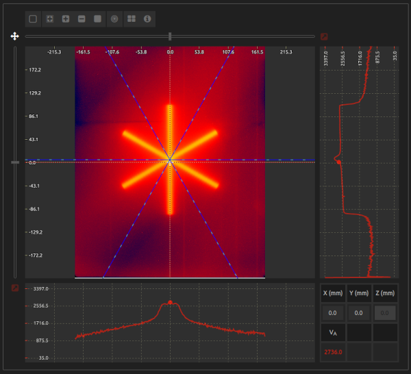
Locate and obtain the dimensions of the radiation isocenter by analyzing a Starshot test.
- Step 1:
- Open MACHINE QA in the menu.
- Step 2:
- Click Starshot.
- Step 3:
- Select an image of a Starshot test.
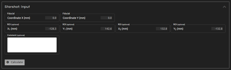
- Step 4 (Inputs):
- Enter the inputs for the calculation:
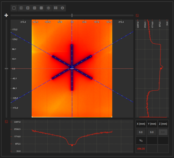
- Polarity detection:
- The axes of the star should have lower values than the background. If this is not the case, click the Complement button on Image / Transform to generate the complementary image. Alternatively, enable Polarity detection to automatically determine the correct image polarity.
- Threshold level:
- Adjust the threshold level if automatic detection of the Starshot pattern is not optimal.
- Marker:
- Lock the cursor by clicking on and use the sliders located at the top and left sides of the canvas to align it with the fiducial/laser isocenter, if marked on the image. Otherwise, lock the cursor in a position near the center of the star.
- ROI (optional):
- Prevent labels and other artifacts from interfering in the calculation by selecting a ROI.
- Comments (optional):
- Add comments if desired.
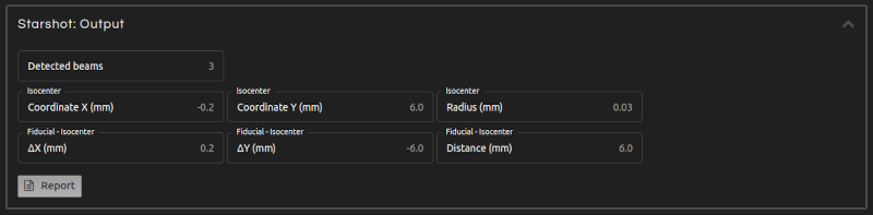
- Step 5 (Outputs):
- Click Calculate. The results will show after a few seconds:
- Isocenter coordinates:
- Position of the radiation isocenter.
- Isocenter radius:
- Radius of the radiation isocenter.
- Marker-isocenter:
- Displacement (marker - isocenter) in X and Y, and distance between the marker and the radiation isocenters.
- Beam angles:
- Beam angles with respect to the coordinate system in the image display.
- Step 6:
- Click Report to get the results in a PDF, CSV, or JSON file.
- Troubleshooting 1:
- The axes of the star have higher values than the background. Click the Complement button on Image / Transform to calculate the complementary image or enable Polarity detection.
- Troubleshooting 2:
- The cursor is far from the center of the star. Lock the cursor in a position closer to the isocenter.
- Troubleshooting 3:
- Excessive noise, large beam widths, beams too close to each other, image artifacts, etc., can induce errors in the location of the beams.
- References:
- Depuydt, T., et al. "Computer-aided analysis of star shot films for high-accuracy radiation therapy treatment units." Physics in Medicine & Biology 57.10 (2012): 2997
- Gonzalez, A., et al. "A procedure to determine the radiation isocenter size in a linear accelerator." Medical physics 31.6 (2004): 1489-1493
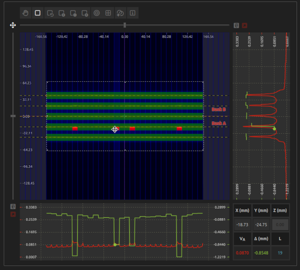
Check the accuracy of MLC positions with the Picket Fence test.
This test is compatible with the analysis of the Bayouth and Hancock tests. It also enables the analysis of Varian Halcyon MLCs on proximal, distal, and both layers.
- Step 1:
- Open MACHINE QA in the menu.
- Step 2:
- Click MLC Picket Fence.
- Step 3:
- Select an image of a Picket Fence test.
- Step 4:
- The beam lines should be horizontal. If this is not the case, transform the image by rotating it.
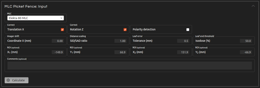
- Step 5 (Inputs):
- Enter the inputs for the calculation:
- MLC:
- Select the MLC model.
- Correct Translation:
- Automatically correct any small offset of the MLC position on the x-axis.
- Correct Rotation:
- Automatically correct any small rotation of the beam lines.
- Polarity detection:
- The beam lines should have higher values than the background. If this is not the case, click the Complement button on Image / Transform to generate the complementary image. Alternatively, enable Polarity detection to automatically determine the correct image polarity.
- Threshold level:
- Adjust the threshold level if automatic detection of the Picket Fence pattern is not optimal.
- Imager shift:
- Enter the offset on the X-axis of the Imager (e.g., EPID) respect to the isocenter, either manually or by locking the cursor near the center of the MLC on the X-axis.
- Distance scaling:
- Introduce distance scaling (i.e., Source to Imager Distance / Source to Axis Distance).
- Tolerance:
- Tolerance for errors of leaf positions.
- Leaf end threshold:
- By default, the leaf end is located at the position of the 50% isodose between the peak of the signal and the background (i.e., the FWHM), which is appropriate when working with doses. You can change the threshold level to locate the leaf end more accurately when pixel values do not correspond to doses (e.g., with EPIDs).
- ROI (optional):
- Delineate the ROI (i.e., the MLC region).
- Comments (optional):
- Add comments if desired.
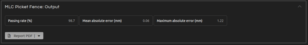
- Step 6 (Outputs):
- Click Calculate. The results will show after a few seconds:
- Passing rate:
- Percentage of leaf positions within tolerance.
- Mean absolute error:
- Mean absolute leaf position error.
- Maximum absolute error:
- Maximum absolute leaf position error.
- Step 7:
- Click Report to get the results in a PDF, CSV, or JSON file.
- Troubleshooting 1:
- The beam lines are vertical. Transform the image by rotating it.
- Troubleshooting 2:
- The beam lines have lower values than the background. Click the Complement button on Image / Transform to calculate the complementary image or enable Polarity detection.
- Troubleshooting 3:
- In the report, the Aperture is not accurate. When pixel values do not correspond to doses (e.g., with EPIDs), you may need to adjust the Leaf End Threshold Level to more accurately locate the leaf end.
- References:
- LoSasso, T. "IMRT delivery system QA." Intensity modulated radiation therapy: the state of the art. Madison, WI: Medical Physics Publishing (2003): 561-91
- Hancock, S, Whitaker, M. "SU-E-T-129: an EPID-based method for testing accuracy of MLC and backup jaws." Medical physics (2013) 40(6 Part12):233
- Bayouth, J.E., et al. "MLC quality assurance techniques for IMRT applications." Medical physics 30 (2003): 743
Evaluate the impact of gravity on the MLC by measuring the output at multiple gantry angles.
This test corresponds to Varian RapidArc QA Test 0.1: DMLC Dosimetry ("RapidArc QA Test Procedures for TrueBeam." Varian Medical Systems, Inc. (2014)).
- Step 1:
- Open MACHINE QA in the menu.
- Step 2:
- Click MLC Dosimetry.
- Step 3:
- Select a Series with a MLC Dosimetry test.
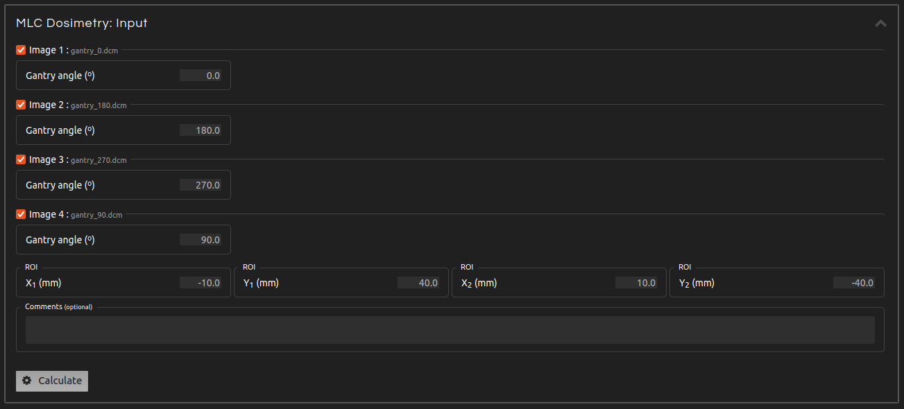
- Step 4 (Inputs):
- Enter the inputs for the calculation if they are not automatically populated from the DICOM file or if they are incorrect. Uncheck the images that you want to exclude from the calculation. The inputs include:
- Gantry angle:
- Introduce the gantry angle for each image.
- ROI:
- Select the ROI inside the field where the output will be measured.
- Comments (optional):
- Add comments if desired.
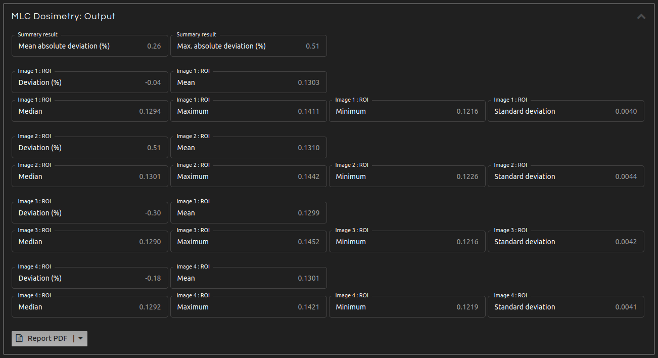
- Step 5 (Outputs):
- Click Calculate. The results will show after a few seconds:
- Summary:
- Mean and maximum absolute percentage deviation.
- Image N: ROI. Deviation:
- Percentage deviation between the mean of the image and the mean of the means of all images.
- Image N: ROI. Mean, median, maximum, minimum, and standard deviation:
- Mean, median, maximum, minimum, and standard deviation of the pixel values inside the ROI of Image N.
- Step 6:
- Click Report to get the results in a PDF, CSV, or JSON file.
- References:
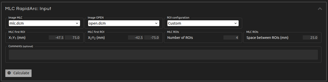
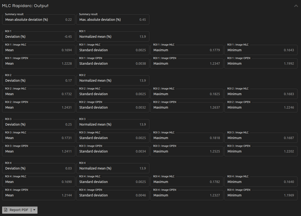
Analyze the control accuracy of dose rate, gantry speed, and leaf speed during RapidArc delivery.
This test corresponds to Varian RapidArc QA Tests 2 and 3 ("RapidArc QA Test Procedures for TrueBeam." Varian Medical Systems, Inc. (2014)).
- Step 1:
- Open MACHINE QA in the menu.
- Step 2:
- Click MLC RapidArc.
- Step 3:
- Select a Series with a MLC RapidArc test.
- Step 4 (Inputs):
- Enter the inputs for the calculation:
- Image MLC:
- Select the image with a field delivered using the MLC.
- Image OPEN:
- Select the image with an open field.
- ROI configuration:
- Select predefined ROI settings or customize your own.
- MLC first ROI:
- Select the first ROI on the left where the output will be measured.
- Number of ROIs:
- Select the number of ROIs to measure.
- Space between ROIs:
- Select the distance between two consecutive ROIs.
- Comments (optional):
- Add comments if desired.
- Step 5 (Outputs):
- Click Calculate. The results will show after a few seconds:
- Summary:
- Mean and maximum absolute percentage deviation.
- ROI N. Deviation:
- Percentage deviation between the normalized mean of the ROI and the mean of the normalized means of all ROIs.
- ROI N. Normalized mean:
- Normalized mean (N) defined as: $$N = 100 \cdot \frac{\overline{MLC}}{\overline{OPEN}}$$
- ROI N. Image MLC:
- Mean, standard deviation, maximum, and minimum of the pixel values inside the ROI N of the Image MLC.
- ROI N. Image OPEN:
- Mean, standard deviation, maximum, and minimum of the pixel values inside the ROI N of the Image OPEN.
- Step 6:
- Click Report to get the results in a PDF, CSV, or JSON file.
- References:
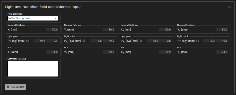
Verify the coincidence of light and radiation field.
- Step 1:
- Open MACHINE QA in the menu.
- Step 2:
- Click Light and radiation field coincidence.
- Step 3:
- Select an image of a Light and radiation field coincidence test.
- Step 4 (Inputs):
- Enter the inputs for the calculation:
- Field definition:
- Select between Inflection points and FWHM. The FWHM follows the standard definition of radiation field as delimited by the 50% isodose of the beam profile. However, this definition requires that films are converted into dose distributions. When working with pixel values, an approximation to the radiation field can be obtained by the inflection points of the profiles.
- Nominal field size:
- Introduce the nominal dimensions of the field on each semiaxis.
- Light points:
- Introduce the points that mark the limits of the light field on each semiaxis. Enable them in Inputs and place them on the canvas.
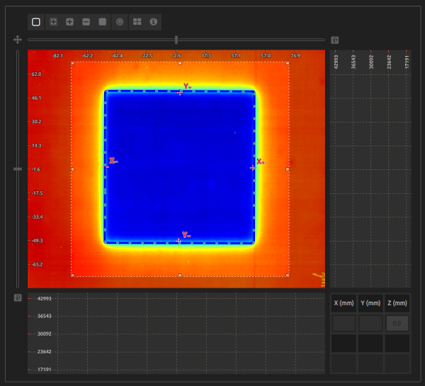
- ROI:
- Select a ROI that encompasses the radiation field.
- Comments (optional):
- Add comments if desired.
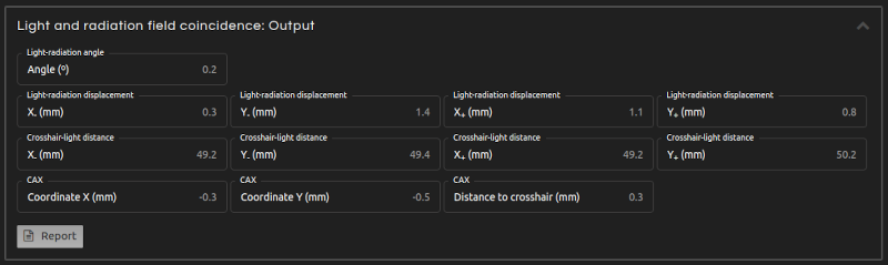
- Step 5 (Outputs):
- Click Calculate. The results will show after a few seconds:
- Light-radiation angle:
- Angle of rotation between light and radiation field.
- Light-radiation displacement:
- Distance between the radiation field and the light field on each semiaxis. It is positive when the radiation field is larger than the light field, and negative when it is smaller.
- Crosshair-light distance:
- Distance between the crosshair and the light field on each semiaxis.
- Crosshair-radiation distance:
- Distance between the crosshair and the radiation field on each semiaxis.
- CAX coordinates (fields with symmetric nominal dimensions only):
- For fields with symmetric nominal dimensions: coordinates of the radiation field center.
- CAX-crosshair distance (fields with symmetric nominal dimensions only):
- For fields with symmetric nominal dimensions: distance between the crosshair and the radiation field center.
- Step 6:
- Click Report to get the results in a PDF, CSV, or JSON file.
- Troubleshooting 1:
- The ROI shall encompass the radiation field, not extend beyond the image, and avoid labels and other artifacts.
- Troubleshooting 2:
- There shall not be any mark on the radiation field apart from the 4 light points. Do not mark the center or the corners of the field.
Analysis of the radiation field, including field size, central dose statistics, flatness, symmetry, penumbra, etc. It can analyze rectangular and circular fields (e.g., cones) of WFF photons, FFF photons, and electron beams.
It is the QA test of choice for measuring small fields and output factors.
Available protocols for flatness and symmetry:
- Photons WFF:
- WFF IEC / Elekta: "IEC 60976. Medical electrical equipment - Medical electron accelerators - Functional performance characteristics." IEC (2007).
- WFF TG45 / Varian: Nath, R., et al. "AAPM code of practice for radiotherapy accelerators: report of AAPM Radiation Therapy Task Group No. 45." Medical Physics 21 (1994): 1093.
- Photons FFF:
- FFF Elekta: "Versa HD Product Data." Elekta AB.
- FFF Varian: "TrueBeam System Specifications." Varian Medical Systems, Inc. (2011)
- FFF AERB of India: Sahani, G., et al. "Acceptance criteria for flattening filter-free photon beam from standard medical electron linear accelerator: AERB task group recommendations." Journal of Medical Physics/Association of Medical Physicists of India 39.4 (2014): 206.
- Electrons:
- Electrons IEC / Elekta: "IEC 60976. Medical electrical equipment - Medical electron accelerators - Functional performance characteristics." IEC (2007).
- Electrons TG45 / Varian: Nath, R., et al. "AAPM code of practice for radiotherapy accelerators: report of AAPM Radiation Therapy Task Group No. 45." Medical Physics 21 (1994): 1093.
- Constancy:
- Flatness and symmetry protocols are defined for dose distributions. If the image does not contain doses (e.g., EPID or film scans), the Constancy protocol allows analysis using pixel values instead. It is intended only for constancy checks. It approximates the radiation field using inflection points and applies the TG45 protocol.
- Step 1:
- Open MACHINE QA in the menu.
- Step 2:
- Click Radiation field.
- Step 3:
- Select an image with a dose distribution of a rectangular or circular radiation field.
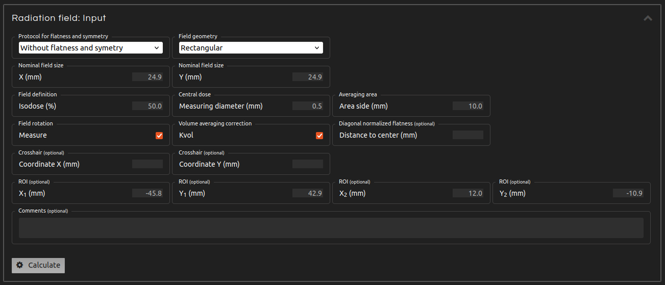
- Step 4 (Inputs):
- Enter the inputs for the calculation:
- Protocol for flatness and symmetry:
- If you want to calculate flatness and symmetry, select one of the available protocols.
- Field geometry:
- Select between rectangular and circular field.
- Nominal field size:
- Nominal field size dimensions.
- Field definition isodose:
- Isodose that delimits the radiation field.
- Central dose diameter:
- Central dose statistics are measured for a circle with this diameter centered on the field.
- Averaging area:
- Side of the area that averages pixel values for flatness and symmetry calculations.
- Correct rotation:
- Correct the rotation of the radiation field. Do not apply rotations on fields with circular symmetry (e.g., cones and very small fields).
- Volume averaging correction:
- Calculate the volume averaging correction (kvol) that should multiply the measured central dose to take into account the dimensions of the central dose diameter. Calculated following the procedure of:
- Diagonal normalized flatness (optional):
- Introduce the distance to the center to calculate the diagonal normalized flatness, as defined in:
- Crosshair coordinates (optional):
- Lock the cursor and align it with the crosshair if the crosshair is marked on the image.
- ROI (optional/mandatory):
- Select a ROI that encompasses the radiation field. This input is mandatory when applying the Constancy or FFF AERB protocols.
- Comments (optional):
- Add comments if desired.
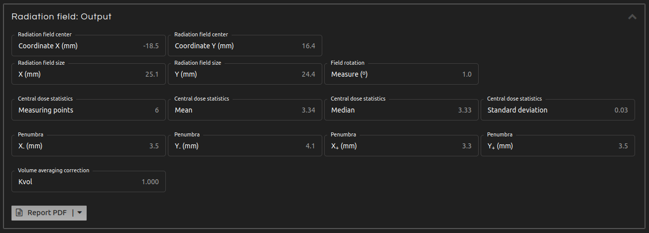
- Step 5 (Outputs):
- Click Calculate. The results will show after a few seconds:
- Radiation field center:
- Coordinates of the center of the radiation field.
- Radiation field size:
- Dimensions of the radiation field.
- Field rotation:
- Rotation of the radiation field.
- Central dose statistics:
- Statistics of the distribution of values within the central dose diameter.
- CAX distance to crosshair:
- If the crosshair is introduced: distance between the crosshair and the central axis.
- Crosshair-field distance:
- If the crosshair is introduced: distance between the crosshair and the field on each semiaxis.
- Penumbras:
- For rectangular fields except for FFF Elekta and FFF Varian: distance between the 80-20% isodoses on each semiaxis.
- Flatness and Symmetry:
- According to the different protocols, the outputs for flatness and symmetry are:
- Photons WFF IEC / Elekta: flatness, symmetry, and maximum ratio of absorbed dose.
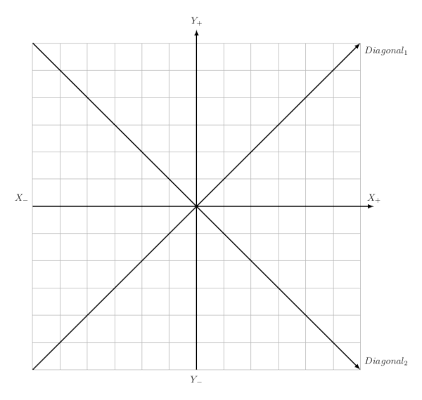
- Photons WFF TG45 / Varian: flatness and symmetry, in both cases on the X and Y axes and both diagonals.
- Photons FFF Elekta: symmetry and isodose values on each semiaxis at different distances from the CAX.
- Photons FFF Varian: flatness, symmetry, isodose values on each semiaxis at different distances from the CAX, distances from the CAX to different isodoses on each semiaxis.
- Photons FFF AERB of India: symmetry and distances from the CAX to different isodoses on each semiaxis.
- Electrons IEC / Elekta: flatness (i.e., distance between the 90% isodose and the edge on each semiaxis and the diagonals), symmetry, and maximum ratio of absorbed dose
- Electrons WFF TG45 / Varian: flatness and symmetry, in both cases on the X and Y axes and both diagonals.
- Constancy: flatness and symmetry, in both cases on the X and Y axes and both diagonals.
- Volume averaging correction:
- Volume averaging correction factor (kvol), if selected.
- Diagonal normalized flatness:
- Diagonal normalized flatness (FDN), if the distance to the center is specified.
- Step 6:
- Click Report to get the results in a PDF, CSV, or JSON file.
- Troubleshooting 1:
- The image must contain a dose distribution to measure flatness and symmetry. Otherwise, use the Constancy protocol, which is intended only for constancy checks.
- Troubleshooting 2:
- Rotation detection may fail if the field has circular symmetry.
- Troubleshooting 3:
- The sample of central dose pixels may be empty if the central dose diameter is too small. As a consequence, the program will return an error.
- Troubleshooting 4:
- If introduced, the crosshair coordinates should be within the ROI.
- References:
- "IEC 60976. Medical electrical equipment - Medical electron accelerators - Functional performance characteristics." IEC (2007).
- Nath, R., et al. "AAPM code of practice for radiotherapy accelerators: report of AAPM Radiation Therapy Task Group No. 45." Medical Physics 21 (1994): 1093.
- Sahani, G., et al. "Acceptance criteria for flattening filter-free photon beam from standard medical electron linear accelerator: AERB task group recommendations." Journal of Medical Physics/Association of Medical Physicists of India 39.4 (2014): 206.
- Casar, B., et al. "A novel method for the determination of field output factors and output correction factors for small static fields for six diodes and a microdiamond detector in megavoltage photon beams." Medical physics 46.2 (2019): 944-963.
- Gao, S., et al. "Measurement of changes in linear accelerator photon energy through flatness variation using an ion chamber array" Medical physics 40.4 (2013): 042101.
Verify the coincidence of the mechanical and radiation isocenters.
- Step 1:
- Open MACHINE QA in the menu.
- Step 2:
- Click Winston-Lutz.
- Step 3:
- Select a series with a Winston-Lutz test. Up to 90 images can be analized.
- Step 4 (Inputs):
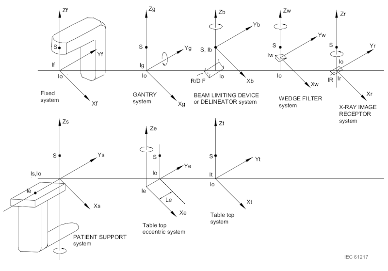
- Enter the inputs for the calculation if they are not automatically populated from the DICOM file or if they are incorrect. The DICOM tags follow the IEC 61217 coordinate system. If necessary, input angles according to this coordinate system. Uncheck the images that you want to exclude from the calculation. The inputs include:
- Threshold level:
- Adjust the threshold level if automatic detection is not optimal.
- SID/SAD ratio:
- Source to Imager Distance / Source to Axis Distance ratio for each image.
- Couch angle:
- Introduce the couch angle for each image.
- Collimator angle:
- Introduce the collimator angle for each image.
- Gantry angle:
- Introduce the gantry angle for each image.
- ROI (optional):
- Crop your image using a ROI to facilitate the detection of the radiation field when it covers less than 1% of the image.
- Comments (optional):
- Add comments if desired.
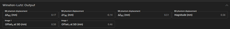
- Step 5 (Outputs):
- Click Calculate. The results will show after a few seconds:
- BB phantom displacement:
- Couch shift needed to align the BB phantom with the radiation isocenter. The displacement is expressed in IEC 61217 coordinates. The magnitude of the displacement (i.e., the distance between the mechanical and radiation isocenters) is also provided.
- Image offsets:
- Offset at SID of each image between the radiation and mechanical isocenters.
- Step 6:
- Click Report to get the results in a PDF, CSV, or JSON file.
- Troubleshooting 1:
- Crop your image using a ROI to facilitate the detection of the radiation field when it covers less than 1% of the image.
- References:

Measure CT and CBCT image quality with automatic Catphan phantom analysis. This test is compatible with Catphan models 500, 503, 504, 600, and 604.
Uniformity and Contrast definitions follow:
- Step 1:
- Open MACHINE QA in the menu.
- Step 2:
- Click Catphan.
- Step 3:
- Select a series with a CT or CBCT scan of a Catphan phantom.
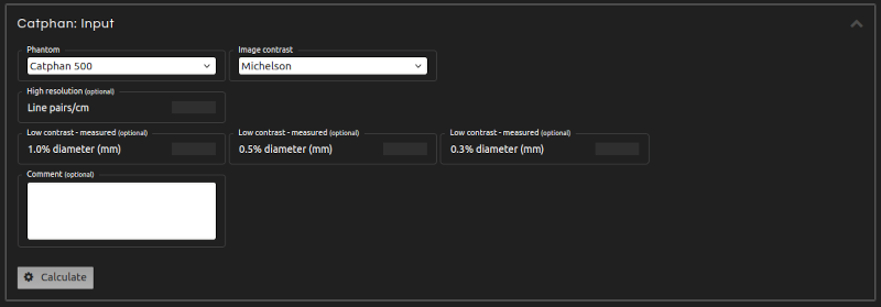
- Step 4:
- Enter the inputs for the calculation:
- Phantom:
- Select the model of the phantom under analysis.
- Image contrast:
- Choose between different definitions of contrast.
- High resolution - observed (optional):
- Optionally, enter the maximum number of line pairs per centimeter that you can discern.
- Low contrast - observed (optional):
- The application automatically analyzes the low contrast module. However, you can also input the dimensions of the targets that you can distinguish across different noise levels.
- Comments (optional):
- Add comments if desired.
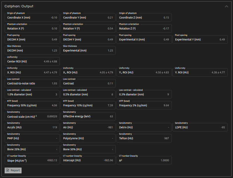
- Step 5 (Outputs):
- Click Calculate. The results will show after a few seconds:
- Origin of phantom:
- DICOM coordinates of the center of the sensitometry module.
- Phantom orientation:
- Rotations of the phantom in each axis.
- Pixel spacing:
- Pixel dimensions as defined in the DICOM files and as measured by the application.
- Slice spacing:
- Slice spacing (i.e., the center-to-center distance between adjacent slices) as defined in the DICOM files and as measured by the application.
- Slice width:
- Slice width (i.e., the reconstructed thickness of each slice) as defined in the DICOM files and as measured by the application.
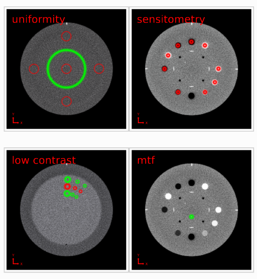
- Uniformity:
- Mean and standard deviation of the Hounsfield Units (HUs) measured in the center of the phantom and in four off-center positions along each semiaxis. The diameter of the ROIs is 10% of the phantom's diameter.
- Noise:
- Standard deviation of the HUs measured in the center of the phantom. The diameter of the ROI is 40% of the phantom's diameter.
- Uniformity index:
- The uniformity index (UI) is characterized by the maximum discrepancy between the mean HUs of the peripheral ROIs and the central ROI of the Uniformity module. $$UI = 100 \cdot \frac{\overline{HU}_{periphery} - \overline{HU}_{center}}{\overline{HU}_{center} + 1000}$$
- Integral non-uniformity:
- Integral non-uniformity (IN) is defined as: $$IN = \frac{\overline{HU}_{max} - \overline{HU}_{min}}{\overline{HU}_{max} + \overline{HU}_{min} + 2000}$$ where \(\overline{HU}_{max}\) and \(\overline{HU}_{min}\) are the maximum and minimum mean HUs in the five ROIs of the Uniformity module.
- Low contrast. ROI and Background:
- Mean and standard deviation of the HUs measured in the target ROIs and local background areas. These areas are shown in the PDF report, with the ROI in red and the background in green.
- Contrast-to-noise ratio:
- The contrast-to-noise ratio (CNR) is defined as: $$CNR = 2 \cdot \frac{|\overline{HU}_{ROI} - \overline{HU}_{background}|}{\sigma_{ROI} + \sigma_{background}}$$
- Contrast:
- Contrast is defined according to the chosen definition as:
- HU difference: $$C = \overline{HU}_{ROI} - \overline{HU}_{background}$$
- Weber: $$C = \frac{\overline{HU}_{ROI} - \overline{HU}_{background}}{\overline{HU}_{background}}$$
- Michelson: $$C = \frac{\overline{HU}_{ROI} - \overline{HU}_{background}}{\overline{HU}_{ROI} + \overline{HU}_{background}}$$
- Low contrast visibility:
- Low contrast visibility is defined from the mean and standard deviation of HUs in the LDPE and polystyrene (PS) targets, if both are present in the Sensitometry module: $$LCV = 2 \cdot \frac{|\overline{HU}_{LDPE} - \overline{HU}_{PS}|}{\sigma_{LDPE} + \sigma_{PS}}$$
- Low contrast - calculated:
- Calculation of the minimum diameters of targets that are detectable at various noise levels. If no target is detectable at a given noise level, the output will not be displayed. The smallest observable diameter is calculated as: $$(\text{smallest diameter}) \cdot CNR \cdot (\text{noise level}) = \text{constant}$$
- MTF:
- Spatial frequencies for different values of the modulation transfer function.
- Sensitometry:
- Analysis of the sensitometry module, including Contrast scale, Effective energy, mean HU, and standard deviation HU values of the target materials.
- CT number linearity:
- Slope, intercept, and coefficient of determination (R²) of the linear fitting of CT numbers as a function of attenuation coefficients of the sensitometry target materials.
- Step 6:
- Click Report to get the results in a PDF, CSV, or JSON file. The PDF report shows the location of the ROIs used in the calculations, showing one slice from each set of aggregated slices.
- Troubleshooting 1:
- The analysis may fail or produce nonsensical results if the selected phantom model is incorrect.
- Troubleshooting 2:
- Pixel and slice dimensions should remain constant throughout the CT scan.
- Troubleshooting 3:
- Neither the slice spacing nor the slice width should exceed 5 mm.
- Troubleshooting 4:
- Jpeg2000 compression is not supported.
- References:
- Catphan 503 Manual. The Phantom Laboratory, Inc. (2017)
- Catphan 500 and 600 Manual. The Phantom Laboratory, Inc. (2015)
- Catphan 604 Manual. The Phantom Laboratory, Inc. (2015)
- Catphan 504 Manual. The Phantom Laboratory, Inc. (2013)
- Elstrøm, U. V., et al. "Evaluation of image quality for different kV cone-beam CT acquisition and reconstruction methods in the head and neck region." Acta Oncologica 50.6 (2011): 908-917.
- Anam, C., et al. "Automated MTF measurement in CT images with a simple wire phantom." Polish Journal of Medical Physics and Engineering 25.3 (2019): 179-187.
- Yin, F-F., et al. "Measurement of the presampling modulation transfer function of film digitizers using a curve fitting technique." Medical physics 17.6 (1990): 962-966.